Basic statistics using Microsoft Excel

Microsoft Excel is a powerful software that have been used my end users and professionals for many years for various purposes. In this post we going to introduce basic statistical features of Excel. This post is using Microsoft Excel 2013, but it is easy to map it to your Excel version.

Basic Formulas

Computations in Excel are carried out using formulas. A formula is a mathematical expression that is used to calculate a value. In Excel, a formula is entered into the active cell by typing an expression. In certain situations, Excel will automatically insert a formula for you.

Excel formulas are always entered beginning with an = sign and followed by the expression. Without an = sign, the expression will be treated as text. The expression will consist of cell references and/or numbers, and contain one or more arithmetic operators such as +, -, *, / or ^. The operator, ^, represents exponentiation. If an expression contains more than one arithmetic operator, the computations are performed in a certain sequence called the order of precedence. The rules in the order of precedence are as follows:

1. Exponentiation (^)
2. Multiplication (*) or Division (/), whichever comes first working from left to right
3. Addition (+) or subtraction (-), whichever comes first working from left to right

If there are any parentheses in the formula, Excel executes the inner most parenthesis first and then works outwards. Within the parenthesis, the order of precedence also holds. Assume you had the following formula in an Excel cell:

=8+(2*(6+5^2*4))

When executed, this formula will enter a value of 220 in that cell. Here is how this value is calculated. First, the inner most parenthesis (6+5^2*4) will be executed. Within this set of parenthesis, the exponentiation will be computed first (5^2=25) to reduce the expression in the inner parenthesis to (6+25*4). Next, the multiplication (25*4=100) is done giving (6+100). This is followed by the addition (6+100=106). This reduces the original formula to =8+(2*106). Next, Excel executes the parenthesis (2*106) giving us 212. Finally, the addition 8+212 is done for a total of 220. Note that if the expression is =8+(2*6+5^2*4), that is without the inner set of parenthesis, the value would be 120.

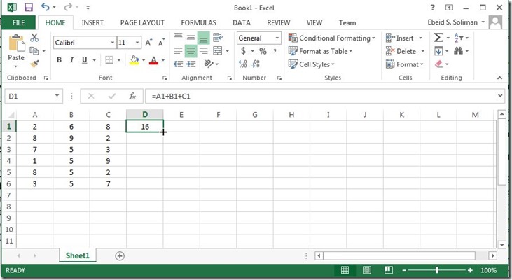
Ways to enter formulas (like A1+B1+C1 ) :

1. Enter the whole formula in the cell that will store the result ( =A1+B1+C1 ) and press Enter.
2. Enter = and then click on cell A1 then enter the + sign using the keyboard then click on cell B1 then enter the + sign using the keyboard then click on cell C1 and press Enter.
3. If the cells to be added are adjacent, you can identify these cells using a range that could be passed to functions. In our case enter =SUM(A1:C2)
4. Many formulas have shortcut command on the Excel ribbon. In our case AutoSum command (represented by the button,, in the Editing group on the Home ribbon tab) is used to sum adjacent horizontal or vertical cells.

In many cases you need to repeat the equation for many cells (e.g. to sum all the rows the in the sheet below)

To repeat the equation for for the rest of D column, you could:

1. Select D1, Copy, select D2, Past, and repeat the operation for the D3, D4, D5, D6
2. Hover the mouse over the left bottom corner of D1 till the curser became small black square (called Fill Handle), then click and drag it to the desired range (D2:D6). Once you release the mouse button, Excel will execute the formula for your range.

You wondering that the equation we copied was for A1+B1+C1, how it worked for the second row and the next rows ? The answer is that Excel automatically adjusted the locations of the cells when the equation was copied from cell D1 to cell D2 since the cells in the expression were all relative reference cells. A relative reference is a cell reference that changes or shifts when the cell is copied to another location. In contrast, an absolute reference is a cell reference that does not change when you copy that cell to another location. There is also a mixed reference for cells. A mixed reference only changes either the row reference or the column reference, depending on how the mixed reference is set up.

All cell references are relative reference cells unless designated otherwise. That is, a cell has to be designated an absolute reference or a mixed reference cell. To create an absolute reference, you have to preface the cell row and column designations with a dollar sign ($). For example, to make Cell A1 an absolute reference cell, it would have to referred as $A$1. Without these dollar prefixes, a cell is always considered a relative location cell. The relative reference works as follows: When you enter the formula, =A1+B1+C1, into Cell D1, the relative location of Cell A1 to Cell D1 is three cells to the left. Similarly, Cell B1 is two cells to the left of Cell D2, and Cell C1 is one cell left. When the equation is copied down to Cell D2, the first cell in this equation will still be the cell three cells to the left. However, the cell three cells to the left of D2 is now Cell A2. Similarly, the cell two cells to the left of D2 is Cell B2, and so on. That is why when the equation is copied down one cell, it makes the automatic adjustment for the new relative locations. Similarly, if the equation is copied down to Cell D3, the equation in Cell D3 would be copied as =A3+B3+C3. If there was an absolute reference cell in this equation, its reference would not change when the equation is copied to another location. The same processing happens when using the Fill Handle.

Basic Functions

Excel have many functions like MIN, MAX, AVERAGE which work on ranges.

Logical Functions

Logic is handled within Excel by logical functions. A logical function is a “logical” statement that determines whether a condition is true or false. Excel has several logical functions. The most commonly used of these is the IF function. The general form of the IF function is: =IF (logical-test, value-if-true, value-if-false)

Example  =IF (A2>=5, “Greater Than 5”, “Less Than 5”)

This function works as follows: logical-test is an expression that is either true or false. If the expression is true, then the expression value-if-true is executed. If the expression is false, then the expression value-if-false is executed. The logical-test is constructed using comparison operators. A comparison operator compares two expressions according to the comparison operator. There are six comparison operators. They are:

• Greater than >
• Less than <
• Equal to =
• Greater than or equal to >=
• Less than or equal to <=
• Not equal to <>

The AND Function

The IF function example above only used one logical test. It can be easily extended to include multiple logical tests. When there are multiple conditions involved, the AND function is used within the IF function as follows: =IF (AND(logical-test 1, logical-test 2, …..), value-if-true, value-if-false)

Each logical-test is an expression that can true or false. If both logical-test 1 and logical-test 2 are true, the AND function returns the value true. Otherwise, it returns the value false. If the AND function returns the value true, the value-if-true expression is executed. If the AND function returns the value false, the value-if-false expression is executed.

Example =IF(AND(A2>=5,B2>=5), “Both A and B Greater than 5”, “Either A or B Less than 5”)

The OR Function

The OR function is also a multiple logical test. When there are multiple conditions involved, the OR function is used within the IF function as follows: =IF (OR (logical-test 1, logical-test 2, …..), value-if-true, value-if-false)

Just like the AND function, each logical-test is an expression that can be true or false. However, with the OR function, if either logical-test 1 or logical-test 2 is true, the OR function returns the value true. If both tests are false, it returns the value false. If the OR function returns the value true, the value-if-true expression is executed. If the OR function returns the value false, the value-if-false expression is executed.

Example =IF(OR(A2>=5,B2>=5), “Either A or B Greater than 5”, “Both A and B Less than 5”)

Lookup

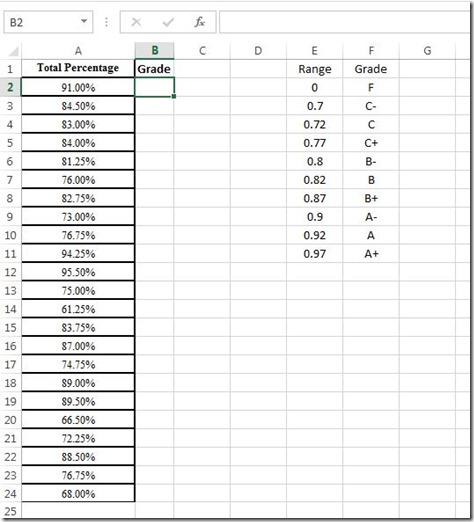
Suppose you want to categorize your data or assign certain classes to your data (like assign class grades based on the total percentage). Excel provides VLOOKUP function. A VLOOKUP function is simply a table with the ranges built in. Excel then matches a data value against these ranges to determine a category or class (grade in our example). To use the VLOOKUP table, you have to first create the VLOOKUP table and then access this VLOOKUP table by using the VLOOKUP function within an Excel statement. The VLOOKUP table can be created anywhere in your sheet. like the one below

Now we need to use the VLOOKUP function to access the VLOOKUP table to assign grades to column B cells. The general form for VLOOKUP is  =VLOOKUP(lookup-value, table-array range, col-index-number, [range lookup])

where:

• lookup-value is the cell reference of the cell that contains the value to be looked up. In this case, the value will be the final percentage scores from the course. That is, the percentage scores in Column O.
• table-array range is the range of the VLOOKUP table. Note that the headers are not included in this range. Also, the range of the table is always entered using absolute references.
• col-index-number is the column number of the value of interest in the VLOOKUP table. For example, in this table, the value of interest is the grade which is in Column 2. Therefore, the col-index-number is 2. If the value of interest is the grade point, then the col-index-number will be 3.
• [range lookup] is an optional argument with a value of true or false. A true value means that look-up value is being evaluated against ranges in the table-array. A false value means that the look-up value must exactly match the value in the table-array. Since this argument is optional, the default value is true.

With the total percentage for the first record in cell A2, the VLOOKUP statement in cell B2 is entered as =VLOOKUP(A2, $E$2:$F$11,2,TRUE)

This statement works as follows: The score in Cell A2 is checked against the first range. Excel forms the first range using the values in Rows 1 and 2 from Column 1 of the VLOOKUP table. These values are 0% and 70%. Therefore, Excel sets the range as 0-70%. Logically, the range is set up as >=0% and <70%. Thus, a score of exactly 70% is not part of this range. If the score from Cell A2 is in this range, a grade of F is returned and recorded in Cell B2. If it is not in this range, Excel forms the second range using the values in Rows 2 and 3 from Column 1. That is, 70% and 72%. As before, this range is set up as >=70% and <72%. If the score is in this range, a grade of C- is returned and recorded in Cell B2. If it is not in this range, Excel forms the third range using the values in Rows 3 and 4 of Column 1 of the VLOOKUP table. That is, 72% and 77%. This range is interpreted as >=72% and <77%. If the score is in this range, a grade of C is returned and recorded in Cell B2. If it is not in this range, Excel continues by forming the fourth range using the values in Rows 4 and 5 of Column 1, and then the fifth range and so on until it finds a range for the score in Cell A2. The last range formed in this table will be 92% to 97% using the values in Rows 9 and 10 of Column 1. If the score is not in this range, then it assigns a grade of A+, the last grade, by default.

To calculate the rest of the grades using this grade criterion, the VLOOKUP function in Cell B2 is copied down to Cell B24.

Basics Of Probability

Probability : a number between 0 and 1 that indicates how likely it is that some event, or set of events, will occur. A probability of 0 indicates it will never occur. A probability of 1 indicates it will always occur. P(event) = 0.2

Experiment : any situation capable of being replicated under essentially stable conditions. The replications may be feasible, such as flipping a coin over and over. Or, the experiment may only replicated in theory, such as investing $1,000 in a friend’s promising invention. In this case you could imagine repeating such an investment over and over many times, even though you intend to do it only once. When an experiment is defined it is important to carefully specify all possible sample outcomes. These are all the possible results of the experiment. For example, if a coin is tossed once, then the sample outcomes are {Head, Tail}. If the experiment is defined as tossing a coin twice, then one way of specifying the sample outcomes would be: {Head, Head}, {Head, Tail}, {Tail, Head}, and {Tail, Tail}. The outcomes of an experiment must be mutually exclusive. Mutually exclusive means there is no overlap between the outcomes. The outcomes of an experiment must also exhaustive. This means one of the defined sample outcomes must occur. There are two basic properties necessary for defining the probability of an outcome:

• 0 ≤ P(Outcome) ≤ 1
•  P(Outcomes) = 1

Probability Rules:

• Rule for Complements: P() = 1 – P(A). represents all sample outcomes except A
• Additive Rule for Mutually Exclusive Events: P(A or B) = P(A) + P(B)
• Joint Probability for Two Independent Events: P(A and B) = P(A)*P(B). Independent means that the occurrence of A have ne influence on the occurrence of B.

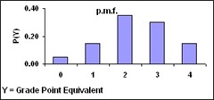
Random Variables : The outcomes of an experiment are said to take place randomly, since they cannot, by definition, occur in any particular order or pattern. Such outcomes, called random variables. Once an experiment and its outcomes have been clearly stated, and the random variable of interest has been defined, then the probability of each value for the random variable can be specified. This specification is called a probability mass function. A probability mass function (p.m.f.) gives the probability for each outcome of a random variable.

Example : Let take a statistics course, receive a grade, letting random variable Y = grade point equivalent.

Outcome	Y	Probability P(Y)
F grade	0	P(Y=0)=0.05
D grade	1	P(Y=1)=0.10
C grade	2	P(Y=2)=0.35
B grade	3	P(Y=3)=0.30
A grade	4	P(Y=4)=0.20

Expected Value : An expected value is the average or mean of a random variable. The expected value of the random variable X is denoted by the symbol E[X], where E[X] = XP(X)

Standard Deviation : The standard deviation of a random variable X measures the average amount by which the values of the random variable X deviate from their expected value. This standard deviation is denoted by σ_X, where σ is the Greek letter sigma.

Discrete random variable: a variable whose values can be separated from one another and counted then the probability of each value for the random variable can be specified. This specification is called a probability mass function.

Continuous random variable: a variable whose values cannot be separated from one another, and are measured rather than counted. Continuous probability distributions are often called probability density functions because it defined over a range of X values (X represents the random variable). The probability that any specific value within this range is so small that it is assumed to be equal zero. Probability P(a < X < b) is the Shaded Area

Determining Normal Probabilities : For data that follow normal distribution this cumulative probability for a normal random variable X P(X<k) is calculated using the following Excel command: =NORM.DIST(k, mean-of-X , Standard-Deviation-of-X,1)

Example: Suppose that the average person’s IQ in US is 100 and the standard deviations for past IQs is 15, then the probability a randomly selected person in the U.S. will have an IQ between 110 and 120 is P(110 < X < 120) = NORMDIST(120,100,15,1)- NORMDIST(110,100,15,1) = 0.9088 - 0.7475 = 0.1613

Normal Inverse : If we want to reverse the previous process, get the X value giving its probability. This is done using the Excel command : =NORM.INV(Probability,mean-of-X , Standard-Deviation-of-X)

Histograms

Histograms allow you to summarize large amounts of data graphically by determining the frequencies over set ranges of specified size (called classes). The width of a class in Excel is called a bin width. The ranges of the classes are called class intervals. The graph of a frequency distribution is called a histogram and is the same as a column chart. To construct a histogram in Excel, we first have to determine the bin width. If you want equal bin widths like the ones below, enter the first and second values (4.20, 4.40), then select both cells and use the fill handle to fill more cells using the same incremental value used in the first two cells  (0.20). In order to create histograms, we need to initialize the analysis toolpak addin that comes with Excel.

Initialize the Analysis Toolpak: Click on the Office button >> Excel Options in the lower right hand corner >> choose the Add-ins section on the left hand side >> click the Go button next to the Manage Excel Add-ins drop down box >> check the box next to Analysis Toolpak and Analysis Toolpak VBA >> press OK.

To create your histogram, go to the Data ribbon tab and click on the Data Analysis button in the Analysis group. In the dialog box that appears, choose Histogram and click Ok. In the resulting dialog table, enter the Input Range (A4:A26), the Bin Range (C2:C15), the worksheet name (histogram1), check the Chart Output option and click on OK. These steps will give a “basic” histogram (like the one below) which can be formatted later.

A common addition to histogram representation, is to convert the frequencies into percentages. For histogram1, calculate the total number of data items by entering a sum function in cell B17. In cell B17, type the formula: =SUM(B2:B16)

Then in cell C2, type the following formula and copy it down to cell C16: = B2/$B$17

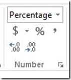
Lastly, format C2:C16 to be percentage with one decimal place. From ribbon Home tab, Number group

In this post we introduced basic statistics operation that can be done easily in Excel. To explain these operations we reviewed some statistics background and general Excel knowledge. In the upcoming posts we will dig deeper using Excel and other specialized software like SAS and R language.